Emergency medical services (EMS) systems face significant challenges in managing fluctuating call volumes, where sudden demand surges can delay response times and worsen outcomes for critical conditions such as cardiac arrest, trauma, and stroke. Accurate forecasting of EMS demand supports proactive ambulance deployment, improving survival rates and resource efficiency, yet traditional methods like ARIMA and exponential smoothing fail to capture nonlinear spatial, temporal, weather, and event-driven effects, and do not provide uncertainty estimates needed for operational decision-making. This paper proposes a conceptual framework based on deep kernel learning with Gaussian processes for spatiotemporal EMS demand forecasting. The model integrates deep neural networks for feature extraction with Gaussian processes for probabilistic inference, enabling both flexible nonlinear representation and uncertainty quantification. It combines temporal, spatial, weather, and event-based kernels to model complex patterns in EMS call volumes. The framework produces predictive mean estimates along with calibrated uncertainty intervals, capturing effects such as weather-driven medical incidents and large public events. This probabilistic output supports risk-aware ambulance allocation strategies that balance over- and under-resourcing. Overall, the proposed approach provides a unified, interpretable, and uncertainty-aware solution for EMS demand forecasting, with future work aimed at validation on real-world datasets and comparison with existing methods.
Emergency medical services systems operate under conditions of substantial demand variability, where call volumes can surge unpredictably due to weather events, holidays, mass gatherings, or disease outbreaks [1, 2]. When call volumes exceed available ambulance capacity, response times increase, leading to worse outcomes for patients with time-sensitive emergencies such as out-of-hospital cardiac arrest, severe trauma, and acute stroke [3, 4]. The economic costs of inefficient ambulance deployment are also substantial, including overtime wages, mutual aid expenses, and increased vehicle wear [5].
Accurate forecasting of EMS call demand enables proactive resource management strategies including ambulance redeployment to high-probability zones, shift staffing adjustments, and preparation for anticipated surge events [6, 7]. Several studies have demonstrated that machine learning approaches can outperform traditional time series methods for EMS demand prediction, particularly when incorporating diverse feature sets including temporal indicators, weather variables, and land use characteristics [1, 8]. However, the operational adoption of these methods remains limited due to concerns about prediction reliability and the lack of uncertainty estimates [9].
Current forecasting approaches face three fundamental limitations when applied to EMS call volume prediction [2, 10]. First, traditional methods such as ARIMA and exponential smoothing assume linear temporal dynamics and cannot capture complex spatial dependencies between neighboring geographic zones [11]. Second, regression-based approaches require manual feature engineering for nonlinear effects of weather and events, which is both labor-intensive and potentially incomplete [12]. Third, most existing machine learning models produce point forecasts without calibrated uncertainty intervals, making it difficult for operations managers to assess prediction confidence and make risk-informed decisions [13].
Table 1 positions the proposed deep kernel learning framework against major EMS forecasting paradigms and clarifies why probabilistic, spatially aware, and automatically learned representations are jointly necessary for operational forecasting.
Table 1. Analytical Positioning of Forecasting Paradigms for EMS Call Volume Prediction
Forecasting paradigm | Representation of temporal dynamics | Representation of spatial dependence | Handling of nonlinear weather and event effects | Uncertainty quantification | Feature engineering burden | Operational interpretability | Principal limitation in EMS deployment | Relative conceptual position of proposed framework |
ARIMA / exponential smoothing | Strong for simple autocorrelation and trend; weak for multi-scale irregular temporal structure | Typically absent or handled indirectly through separate models | Poor; nonlinearities must be imposed externally and remain rigid | Limited; usually interval estimates rely on model assumptions that do not incorporate heterogeneous inputs well | Low to moderate | High for simple time-series behavior | Cannot jointly model rich spatial, weather, and event structure; limited suitability for heterogeneous EMS environments | Baseline temporal benchmark that the proposed framework is designed to exceed |
Conventional regression models | Moderate when lag terms are manually specified | Weak unless spatial covariates are engineered explicitly | Moderate only through handcrafted interactions and polynomial terms | Often incomplete or assumption-sensitive | High | Moderate | Performance depends heavily on manually selected transformations and interactions, making complex event-weather-demand structure difficult to capture | Useful comparator for testing whether automatic feature learning adds value |
Standard machine learning point forecasters (e.g., random forests, gradient boosting, deep networks) | Strong if sufficient lagged features are supplied | Moderate when spatial features are included, but often not structurally encoded | Strong predictive flexibility | Usually weak or indirect; uncertainty often ad hoc, uncalibrated, or unavailable | Moderate | Moderate to low, depending on model complexity | Can improve accuracy but often fail to provide calibrated uncertainty for resource-risk decisions | Demonstrates why predictive accuracy alone is insufficient for EMS operations |
Standard Gaussian process models | Strong for smooth temporal structure if kernels are well designed | Strong when spatial kernels are specified | Moderate; limited by raw-feature representation and kernel expressiveness in high-dimensional heterogeneous settings | Strong; posterior predictive variance is intrinsic | Moderate to high, because kernel design over raw inputs is demanding | High at the kernel level | Scalability and limited raw-feature flexibility can restrict performance in complex multimodal settings | Provides the probabilistic backbone retained by the proposed framework |
Proposed deep kernel learning Gaussian process framework | Strong across short-term lags, periodicity, and longer-range structure through combined feature learning and kernel design | Strong through explicit spatial kernels and information sharing across neighboring or similar zones | Strong; nonlinear transformations are learned automatically while event-weather interactions can be encoded in the composite kernel | Strong and decision-relevant; predictive distributions, credible intervals, and exceedance probabilities are produced natively | Lower than handcrafted nonlinear models, though still design-sensitive | High at the framework level because kernels, outputs, and decision use are structurally aligned | Requires computational approximations, high-quality multisource data, and careful model validation | Integrates expressive representation learning with principled uncertainty quantification for risk-aware EMS forecasting |
Emergency medical services dispatch data exhibit multiple hierarchical temporal patterns that must be captured by any forecasting framework [1, 3]. At the daily level, call volumes typically peak during daytime hours and trough during overnight periods, while weekly patterns show differences between weekdays and weekends corresponding to activity patterns and alcohol consumption [2]. Seasonal variations also emerge, with winter months showing increased respiratory and cardiac emergencies, while summer months see more trauma from outdoor activities and heat-related illnesses [4].
Spatially, EMS call demand is not uniformly distributed across a jurisdiction but rather concentrated in specific hotspots corresponding to population density, commercial activity, elderly care facilities, and high-risk infrastructure [5, 6]. These spatial distributions exhibit temporal dynamics as well, with daytime hotspots near workplaces and nighttime hotspots near residential areas [7]. The granularity of spatial aggregation—whether census tracts, grid cells, or administrative districts—affects both forecasting accuracy and computational tractability, representing a design trade-off in any operational system [8].
Extreme temperatures have been consistently associated with increased EMS dispatches across multiple studies, with both heat waves and cold spells elevating the risk of cardiovascular and respiratory emergencies [4, 7]. The relationship between temperature and call volume is nonlinear, with thresholds beyond which risk increases disproportionately, and these thresholds vary by geographic region and population acclimatization [9, 10]. Lagged effects are also important, as the impact of extreme temperatures may persist for one to several days following the exposure period [11].
Precipitation and air quality represent additional meteorological drivers of EMS demand with complex directional effects [12, 13]. Rainfall typically reduces traffic volumes and thus traffic accident-related calls, but increases the risk of falls among elderly populations and may exacerbate certain respiratory conditions [14]. Fine particulate matter and ozone concentrations show positive associations with dispatches for respiratory emergencies, asthma exacerbations, and psychiatric emergencies, with effect sizes that vary by pollutant source and concentration [15, 16].
Mass gatherings including concerts, sporting events, religious festivals, and political protests generate predictable surges in EMS call volume that can overwhelm local ambulance resources if not anticipated [8, 17]. The magnitude of event-related demand depends on multiple factors including expected attendance, event duration, ambient temperature, alcohol availability, and the demographic profile of attendees [18]. Systematic reviews have documented increased EMS utilization during events ranging from marathon races to music festivals, with call types dominated by minor trauma, dehydration, alcohol intoxication, and exacerbations of chronic conditions [19].
Beyond planned mass gatherings, other calendar events including public holidays, school breaks, and major television broadcasts also influence EMS demand patterns [20, 21]. New Year's Eve consistently shows elevated call volumes related to alcohol consumption and fireworks injuries, while national holidays may show reduced non-emergency calls as routine activities decrease [17]. The integration of event calendars into forecasting models requires encoding of event characteristics—type, size, location, duration—as predictive features that interact with baseline temporal patterns [22].
A Gaussian process defines a distribution over functions, where any finite collection of function values follows a multivariate Gaussian distribution, making it a powerful tool for Bayesian nonparametric regression [10, 11]. The behavior of a Gaussian process is determined by its mean function and covariance function (kernel), where the kernel encodes prior beliefs about the properties of the unknown function such as smoothness, periodicity, and length scales [12]. For spatiotemporal forecasting, Gaussian processes offer the distinct advantage of producing predictive distributions that include both mean forecasts and calibrated uncertainty estimates derived from the posterior covariance [13].
Deep kernel learning extends the Gaussian process framework by parameterizing the kernel function with a deep neural network, learning a transformation of the input space into a feature space where a base kernel is applied [14, 23]. Formally, the deep kernel is defined as k(f_θ(x), f_θ(x')), where f_θ is a deep neural network with parameters θ and k is a standard kernel such as the squared exponential or Matérn [24]. This approach combines the expressive power of deep learning for feature extraction with the probabilistic foundations and uncertainty quantification of Gaussian processes, addressing the limitations of each method when used in isolation [25, 26].
The proposed framework takes as inputs three categories of data: historical EMS dispatch records aggregated by time and spatial zone; meteorological observations and forecasts including temperature, precipitation, humidity, and air quality indices; and public event calendars with information on event type, location, expected attendance, and duration [1, 2]. These heterogeneous inputs are preprocessed into a unified feature vector for each time-spatial unit, including temporal encodings (hour of day, day of week, month), lagged call volumes, weather variables, and event indicators [3]. The deep kernel Gaussian process then learns a mapping from these feature vectors to expected call volume, producing both a point forecast and a predictive variance for each prediction [4].
Figure 1 illustrates the full conceptual architecture of the proposed deep kernel learning framework, showing how heterogeneous spatiotemporal EMS inputs are transformed into probabilistic forecasts and translated into risk-aware operational decisions.
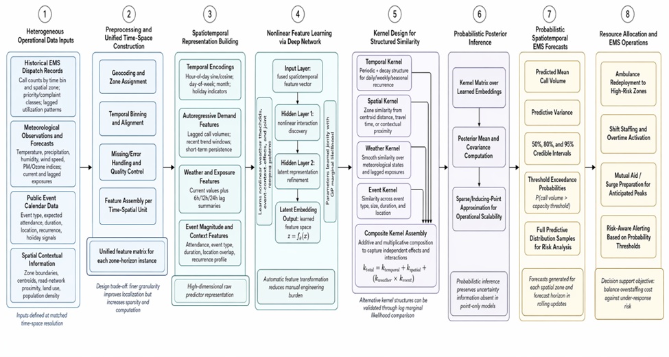
Figure 1. Architecture of the Deep Kernel Learning Framework for Probabilistic Spatiotemporal Forecasting of EMS Call Volume
The output of the framework consists of probabilistic forecasts for each spatial zone and forecast horizon, including mean predicted call volume, credible intervals at specified confidence levels (e.g., 50%, 80%, 95%), and full predictive distributions that can be sampled for risk analysis [5, 6]. These outputs are designed to support operational decision-making, enabling EMS managers to answer questions such as "What is the probability that Zone A will experience more than five calls in the next hour?" [7]. The framework is designed for rolling forecasting, where predictions are updated as new data become available, allowing dynamic redeployment decisions [8].
The framework assumes that historical EMS dispatch data of sufficient quality and duration are available for model training, with a minimum recommended training period of two years to capture seasonal patterns and multiple instances of event types [2, 9]. It further assumes that weather forecasts with adequate accuracy are accessible in real time, and that event calendars are maintained with sufficient lead time to enable proactive resource allocation [10]. The spatial structure of EMS demand is assumed to be relatively stable over the forecasting horizon, though gradual changes due to population shifts or land use changes may require periodic model retraining [11].
Several additional assumptions underlie the Gaussian process component of the framework, including that the latent function governing call volume is smooth in the learned feature space and that the observation noise is Gaussian [12, 13]. The framework assumes that spatial zones are defined in a way that respects natural boundaries and population distributions, though the specific zone definition may vary by jurisdiction and data availability [14]. Finally, the framework assumes that event-related demand is additive to baseline demand rather than multiplicative, an assumption that can be relaxed through alternative kernel constructions [15].
The framework is guided by four design principles that prioritize practical utility for EMS operations [1, 16]. First, probabilistic prediction is emphasized over point forecasting alone, as operational decisions require calibrated uncertainty estimates to balance risks and costs appropriately [17]. Second, spatial correlation is modeled explicitly rather than treating each zone independently, enabling information sharing between neighboring zones and improving predictions for data-sparse areas [18]. Third, the framework incorporates automatic nonlinear feature learning through the deep neural network component, reducing the burden of manual feature engineering for weather and event effects [19]. Fourth, the framework is designed for computational tractability in operational settings, with approximations such as inducing point methods available to address the cubic scaling of exact Gaussian process inference [20].
The base kernel within the deep kernel learning framework provides the foundational similarity measure in the transformed feature space, with the squared exponential kernel serving as a default choice for smooth, infinitely differentiable functions [10, 11]. The squared exponential kernel is defined as
Beyond stationary kernels, periodic kernels capture repeating patterns in EMS demand such as daily, weekly, and annual cycles that are fundamental to dispatch data [14, 24]. The periodic kernel is defined as
The deep neural network component of the framework learns a nonlinear transformation from raw input features to a latent representation where a stationary kernel can effectively measure similarity [23, 24]. The network architecture typically consists of multiple hidden layers with rectified linear unit or hyperbolic tangent activation functions, with the output dimension determining the dimensionality of the transformed feature space [25]. Input features include temporal encodings (hour of day encoded as sine/cosine pairs, day of week indicators, month indicators), weather variables (temperature, precipitation, humidity, wind speed, air quality index), event indicators (binary or continuous event magnitude), and lagged call volumes [1, 26].
The parameters of the deep neural network are learned jointly with the kernel hyperparameters by maximizing the log marginal likelihood of the Gaussian process, which provides automatic regularization against overfitting [27, 28]. This joint optimization balances the expressiveness of the deep feature extractor against the simplicity of the base kernel, learning features that are relevant for the prediction task while maintaining the probabilistic interpretation of the Gaussian process [10, 11]. Dropout and weight decay techniques can be applied during training to improve generalization and prevent the network from learning spurious patterns specific to the training data [12].
The composite kernel combines multiple kernel functions through addition and multiplication to capture different aspects of EMS demand variation simultaneously [13, 14]. The additive composition
Multiplicative kernel compositions, where
The spatial kernel component captures similarity between different geographic zones based on their locations, enabling information sharing across neighboring areas [1, 2]. A simple approach uses Euclidean distance between zone centroids within a squared exponential kernel, such that zones that are geographically close have higher covariance than distant zones [3]. However, for EMS applications, road network distance or travel time may be more appropriate than Euclidean distance, as emergency response and patient transport follow road networks rather than straight-line paths [4].
The spatial length scale parameter determines how quickly spatial correlation decays with distance, and this parameter can be learned from the data or allowed to vary across the region [5, 6]. For large jurisdictions with heterogeneous geography, a spatially-varying length scale may be appropriate, with shorter correlation distances in dense urban areas and longer distances in rural areas [7]. The spatial kernel can also incorporate population density or land use information as additional inputs, encoding the expectation that zones with similar demographic or built environment characteristics have similar EMS demand patterns even if they are not geographically adjacent [8].
Temporal dependencies in EMS call volume are captured through a combination of explicit temporal features in the deep neural network and autoregressive structure in the kernel [9, 10]. The deep network receives as inputs the hour of day, day of week, and month encoded as periodic variables, allowing it to learn the complex diurnal and weekly patterns characteristic of EMS demand [11]. Additionally, lagged call volumes from previous time steps can be included as input features, providing an autoregressive component that captures short-term persistence and momentum in call patterns [12].
For longer-range temporal dependencies, the kernel can include a temporal covariance component that decays with time separation, such that calls that occurred far in the past have less influence on current predictions than recent calls [13, 14]. This temporal decay can be combined with the periodic kernel to capture patterns that repeat daily or weekly while still allowing the influence of any single past observation to diminish over time [15]. The combination of learned deep features and explicit temporal kernel structures provides a flexible yet interpretable approach to modeling the complex temporal dynamics of EMS demand [16].
The Gaussian process formulation provides predictive distributions that include both mean predictions and posterior variances, enabling principled uncertainty quantification for EMS forecasts [17, 18]. The predictive variance at any test point depends on the proximity of that point to training data in the learned feature space, with predictions in regions of sparse data receiving higher uncertainty [19]. This property is particularly valuable for EMS applications, where predictions for unusual combinations of conditions—such as an extreme weather event coinciding with a major public gathering—should be treated with appropriate caution [20].
The predictive distribution can be used to construct credible intervals at any desired confidence level, such as the 50%, 80%, or 95% intervals that might inform different operational decisions [21, 22]. For ambulance redeployment, a 50% credible interval might be sufficient for routine adjustments, while a 95% interval would be more appropriate for triggering surge preparations [23]. Full predictive distributions can also be sampled to support risk-based optimization, such as minimizing the expected cost of under-responding given asymmetric costs of overstaffing versus understaffing [1].
Raw EMS dispatch records require substantial preprocessing before they can be used for deep kernel learning [1, 2]. Each call record must be geocoded to an assigned spatial zone, timestamped to the appropriate temporal bin (typically hourly), and classified by call priority or complaint type if such distinctions are relevant to the forecasting task [3]. Missing or erroneous data—including incomplete addresses, incorrect timestamps, or duplicate records—must be handled through imputation or exclusion based on predefined quality thresholds [4].
The choice of spatial and temporal aggregation granularity represents a fundamental design trade-off in the framework [5, 6]. Finer spatial resolution (e.g., grid cells of 500 meters versus census tracts) provides more precise location information but increases data sparsity and computational complexity, while coarser resolution reduces variance but obscures localized patterns [7]. Similarly, hourly aggregation captures diurnal patterns but may be too coarse for real-time redeployment decisions, whereas 15-minute aggregation provides finer resolution but increases noise [8].
Weather data must be aligned with the same spatial and temporal resolution as the dispatch data, typically by assigning to each zone the nearest weather station observation or interpolated grid value [9, 10]. Key meteorological variables for EMS forecasting include temperature (current, minimum, maximum), precipitation type and intensity, relative humidity, wind speed, and air quality indices for particulate matter and ozone [11, 12]. Lagged weather effects require constructing features for multiple time windows, such as the temperature averaged over the past 6, 12, and 24 hours, as the impact of heat or cold may persist beyond the immediate observation period [13].
The nonlinear relationship between weather variables and EMS demand motivates the use of deep learning to automatically discover appropriate transformations rather than relying on manually specified thresholds or polynomial terms [14, 15]. Extreme weather conditions that occur rarely in the training data will receive appropriately high predictive uncertainty from the Gaussian process, reflecting the model's limited experience with such conditions [16]. Weather forecasts for future time horizons can be substituted for observed weather during prediction, with the understanding that forecast errors will propagate into prediction uncertainty [17].
Public events data require encoding of event characteristics that influence EMS demand, including event type (sports, concert, festival, protest), expected attendance, duration, location zone, and temporal pattern (whether the event occurs on a single day or spans multiple days) [18, 19]. For recurring events such as weekly sports matches, historical call data from previous occurrences can inform the expected demand surge, while novel events must rely on event characteristics and analogous events [20]. The timing of events relative to baseline temporal patterns matters substantially, as a concert on a Saturday evening will have different marginal impact than the same concert on a Tuesday afternoon [21].
Event attendance estimates can be treated as uncertain inputs, with the Gaussian process framework naturally accommodating input uncertainty through modifications to the predictive distribution [22, 23]. Multiple events occurring simultaneously in the same spatial zone may have synergistic effects on EMS demand that exceed the sum of individual event impacts, requiring interaction terms in the composite kernel [1, 2]. Post-event analysis of prediction errors can identify systematic under- or over-prediction for specific event types, enabling iterative refinement of event feature encodings [3].
Probabilistic forecasts enable dynamic ambulance redeployment strategies that move idle vehicles from low-demand zones to areas with high predicted call volume [4,5]. Unlike deterministic redeployment rules that respond only to current queue lengths, forecast-driven redeployment anticipates future demand surges and positions resources before they are needed [6]. The predictive variance from the Gaussian process allows risk-averse redeployment that only moves ambulances when the probability of exceeding a threshold exceeds a specified confidence level [7].
Table 2 shows how each probabilistic output of the framework can be translated into concrete EMS operational decisions, thereby linking model design to redeployment, surge preparation, and threshold-based alerting.
Table 2. Translation of Probabilistic Forecast Outputs into EMS Operational Decision Logic
Forecast output component | What the output represents | Operational question supported | Decision mechanism enabled | Example EMS action | Strategic value | Key implementation caution |
Predictive mean call volume | Expected call demand for a given zone and forecast horizon | Where is demand most likely to increase next? | Baseline demand ranking across zones | Reposition idle ambulances toward the highest-mean demand areas | Improves proactive positioning under routine conditions | Mean alone may understate tail risk during unusual conditions |
Predictive variance | Model uncertainty associated with the forecast | How confident is the system about this predicted surge? | Confidence-sensitive filtering of actions | Delay aggressive redeployment when uncertainty is very high or request supervisory review | Prevents overreaction to unstable predictions | High variance may reflect sparse data rather than genuinely volatile demand |
Credible intervals (50%, 80%, 95%) | Range of plausible call volumes at different confidence levels | What level of preparedness is justified under different risk tolerances? | Multi-threshold planning by confidence level | Use 50% intervals for routine adjustments and 95% intervals for surge contingency planning | Aligns operational response intensity with uncertainty tolerance | Wide intervals may reduce decisiveness unless tied to explicit policy rules |
Threshold exceedance probability | Probability that demand will surpass a predefined capacity or workload threshold | What is the chance that current ambulance capacity will be insufficient? | Probability-triggered alerting and escalation | Activate surge staffing if probability of exceeding ten calls in the next hour crosses a preset threshold | Converts forecasts into actionable alert rules | Thresholds must be calibrated to local fleet size, staffing, and tolerance for false alarms |
Full predictive distribution samples | Distributional scenarios across the full uncertainty range | What are plausible best-case, typical, and worst-case demand realizations? | Scenario-based resource planning and simulation | Stress-test dispatch plans against upper-tail demand realizations before a festival or severe weather period | Supports robust planning under asymmetric under-response costs | Requires simulation-ready operational infrastructure and decision protocols |
Spatially differentiated forecasts across zones | Joint risk distribution across neighboring or functionally similar areas | Could a surge in one zone spill into adjacent operational areas? | Coordinated multi-zone redeployment logic | Stage backup units at boundary zones serving several at-risk areas | Enhances system-wide rather than siloed response planning | Benefits depend on accurate spatial zoning and realistic correlation structure |
Rolling forecast updates | Forecast refresh as new calls, weather, and event information arrive | Should previously planned redeployment or surge measures be revised now? | Dynamic revision of operational stance | Update fleet distribution every hour as incoming data change risk estimates | Maintains responsiveness in evolving demand environments | Frequent updates can create operational churn unless update cadence is governed |
Forecast-informed asymmetric cost framing | Uses uncertainty outputs to weigh under-response against overstaffing differently | Which deployment policy minimizes operational risk rather than error alone? | Cost-sensitive resource allocation | Accept some overcoverage during high-consequence events to reduce catastrophic under-response | Brings the model into direct alignment with EMS service objectives | Requires explicit managerial agreement on cost asymmetry and service priorities |
The operational value of probabilistic forecasts can be quantified through simulation of dispatch policies, comparing expected response times under forecast-driven redeployment versus baseline strategies [8, 9]. Spatial correlation in the forecasts enables coordinated redeployment across zones, recognizing that a surge in one zone often precedes surges in neighboring zones [10]. Real-time implementation requires integration with ambulance tracking systems and dispatch software, with forecasts updated continuously as new call and weather data arrive [11].
Beyond routine redeployment, probabilistic forecasts support surge preparation for anticipated high-demand periods such as holidays, extreme weather events, or major public gatherings [12, 13]. When the predicted call volume for a zone exceeds available ambulance capacity with high probability, operations managers can activate contingency plans including calling in overtime staff, recalling off-duty crews, or requesting mutual aid from neighboring jurisdictions [14]. The lead time of forecasts determines which interventions are feasible, with longer lead times enabling staffing adjustments and shorter lead times supporting real-time redeployment [15].
Threshold-based alerting systems can be constructed from the predictive distribution, generating notifications when the probability of exceeding a critical call volume surpasses a predefined risk tolerance [16, 17]. For example, an alert might trigger when the forecast probability of more than ten calls in a zone over the next hour exceeds 80%, with the threshold calibrated to local resource constraints [18]. Post-event review of forecast performance against actual demand provides feedback for continuous improvement of both the forecasting model and the alerting thresholds [19].
Evaluation of probabilistic forecasts requires metrics that assess both point forecast accuracy and probabilistic calibration [20, 21]. For point forecasts, mean absolute error and root mean squared error measure average prediction accuracy, though these metrics ignore uncertainty estimates entirely [22]. The continuous ranked probability score (CRPS) evaluates the entire predictive distribution, penalizing forecasts that are either inaccurate or overconfident [23, 24]. A perfectly calibrated forecast has the property that actual observations fall within the x% credible interval approximately x% of the time across many predictions [1].
Additional metrics specific to operational decision-making include the area under the receiver operating characteristic curve for threshold exceedance predictions and the expected cost of prediction errors under asymmetric loss functions [2, 3]. For EMS applications, underestimating demand (leading to insufficient resources) typically carries higher cost than overestimating demand (leading to idle ambulances), motivating evaluation under weighted scoring rules [4]. Forecast sharpness—the narrowness of prediction intervals—is also desirable, as overly wide intervals provide little decision-relevant information even if well-calibrated [5].
Temporal cross-validation is essential for time series forecasting, as random splitting of data would leak future information into the training set and produce overly optimistic performance estimates [6, 7]. A standard approach trains on two or more years of historical data and tests on the subsequent year, rolling the training window forward to evaluate performance across multiple test periods [8]. This protocol respects the temporal order of observations and provides realistic estimates of out-of-sample forecast accuracy [9].
Spatial validation examines whether the model generalizes to geographic zones not seen during training, which is relevant for deployment to new jurisdictions [10, 11]. Leave-one-zone-out cross-validation trains on all but one spatial zone and tests on the held-out zone, measuring the model's ability to transfer learned patterns across similar geographic areas [12]. Event holdout validation excludes all instances of a particular event type (e.g., all concerts) from training and tests on held-out concerts, assessing whether event effects generalize across different venues and attendance levels [13].
This paper has presented a conceptual framework for probabilistic spatiotemporal forecasting of emergency medical services call volume based on deep kernel learning with Gaussian processes. The framework addresses key limitations of existing approaches by providing calibrated uncertainty estimates alongside point forecasts, modeling spatial correlations between neighboring zones, and automatically learning nonlinear relationships between weather, events, and EMS demand. The composite kernel structure allows explicit encoding of different sources of variation while maintaining the probabilistic foundations and interpretability of the Gaussian process.
The primary advantages of the proposed framework include its principled handling of uncertainty, which enables risk-aware operational decision-making for ambulance redeployment and surge preparation. The deep feature extractor reduces the burden of manual feature engineering, automatically discovering relevant transformations of temporal, weather, and event inputs. The spatial kernel component enables information sharing across geographic zones, improving predictions for data-sparse areas and capturing the spatial propagation of demand surges.
Several limitations must be acknowledged, including the computational challenges of scaling Gaussian processes to large datasets, the dependence on high-quality event calendar data, and the complexity of model optimization and interpretation. Sparse approximations and stochastic variational inference provide pathways to practical implementation, but these approximations introduce trade-offs between computational efficiency and predictive accuracy. The arbitrary definition of spatial zones and the need for periodic model retraining represent additional practical considerations for deployment.
Future work should focus on implementation of the framework on public EMS datasets such as the National Emergency Medical Services Information System (NEMSIS) or similar regional data sources, enabling empirical comparison with baseline methods including ARIMA, exponential smoothing, long short-term memory networks, and standard Gaussian processes. Sensitivity analyses examining the impact of spatial zone resolution, temporal aggregation, and inducing point count on forecast accuracy and computational requirements would inform practical deployment guidelines. Ultimately, prospective validation in operational settings, with real-time forecasting integrated into dispatch systems, is needed to demonstrate the framework's impact on response times and patient outcomes.
None
None
None
None
Open Access The author(s) retain copyright. This article is licensed under the Creative Commons Attribution-NonCommercial-ShareAlike 4.0 International License. It may be shared and adapted for non-commercial purposes with appropriate attribution, an indication of changes, and distribution of adaptations under the same license. Third-party material may be subject to separate terms identified in its credit line. View the license at https://creativecommons.org/licenses/by-nc-sa/4.0/.
 Clinical Intelligence Research Press